Polars is a "lightning-fast DataFrame library for Rust and Python" - if you're familiar with Pandas, Polars is quite similar but significantly faster and with a cleaner API. This post is a brief tour of how to set up and use Polars, working through a pragmatic example of the things you might do in a typical data exploration project.
The Setup
Install polars and jupyter:
python3 -m venv venv
source venv/bin/activate
pip install polars notebook
This sets up a python virtual environment, then installs the Polars library as well as jupyter. The page you're looking at was created as a jupyter notebook.
The Data
I'm using the New York Taxi Dataset parquet files in this notebook. I downloaded the October 2022 Yellow Taxi Trip Records (PARQUET) file, feel free to grab that as well.
The data is in parquet format, which is quite a nice format for data processing, significantly better than CSV.
Polars
Let's import polars and read the file:
import polars as pl
fname = "yellow_tripdata_2022-10.parquet"
data = pl.read_parquet(fname)
Let's see what it looks like
data.head(5)
| VendorID | tpep_pickup_datetime | tpep_dropoff_datetime | passenger_count | trip_distance | RatecodeID | store_and_fwd_flag | PULocationID | DOLocationID | payment_type | fare_amount | extra | mta_tax | tip_amount | tolls_amount | improvement_surcharge | total_amount | congestion_surcharge | airport_fee |
|---|---|---|---|---|---|---|---|---|---|---|---|---|---|---|---|---|---|---|
| i64 | datetime[ns] | datetime[ns] | f64 | f64 | f64 | str | i64 | i64 | i64 | f64 | f64 | f64 | f64 | f64 | f64 | f64 | f64 | f64 |
| 1 | 2022-10-01 00:03:41 | 2022-10-01 00:18:39 | 1.0 | 1.7 | 1.0 | "N" | 249 | 107 | 1 | 9.5 | 3.0 | 0.5 | 2.65 | 0.0 | 0.3 | 15.95 | 2.5 | 0.0 |
| 2 | 2022-10-01 00:14:30 | 2022-10-01 00:19:48 | 2.0 | 0.72 | 1.0 | "N" | 151 | 238 | 2 | 5.5 | 0.5 | 0.5 | 0.0 | 0.0 | 0.3 | 9.3 | 2.5 | 0.0 |
| 2 | 2022-10-01 00:27:13 | 2022-10-01 00:37:41 | 1.0 | 1.74 | 1.0 | "N" | 238 | 166 | 1 | 9.0 | 0.5 | 0.5 | 2.06 | 0.0 | 0.3 | 12.36 | 0.0 | 0.0 |
| 1 | 2022-10-01 00:32:53 | 2022-10-01 00:38:55 | 0.0 | 1.3 | 1.0 | "N" | 142 | 239 | 1 | 6.5 | 3.0 | 0.5 | 2.05 | 0.0 | 0.3 | 12.35 | 2.5 | 0.0 |
| 1 | 2022-10-01 00:44:55 | 2022-10-01 00:50:21 | 0.0 | 1.0 | 1.0 | "N" | 238 | 166 | 1 | 6.0 | 0.5 | 0.5 | 1.8 | 0.0 | 0.3 | 9.1 | 0.0 | 0.0 |
What are the columns in this file?
data.columns
['VendorID',
 'tpep_pickup_datetime',
 'tpep_dropoff_datetime',
 'passenger_count',
 'trip_distance',
 'RatecodeID',
 'store_and_fwd_flag',
 'PULocationID',
 'DOLocationID',
 'payment_type',
 'fare_amount',
 'extra',
 'mta_tax',
 'tip_amount',
 'tolls_amount',
 'improvement_surcharge',
 'total_amount',
 'congestion_surcharge',
 'airport_fee']
Pretty easy to guess what the columns mean.
Let's poke around a little bit - what's the average taxi fare in NYC?
data["total_amount"].mean()
22.247540895418666
I wonder how many passengers there are in each ride?
data["passenger_count"].mean()
1.3846936672698376
How about the average fare from the airport? I noticed the airport_fee column, let's look at average total_amount when the airport fee is greater than zero:
data.filter( pl.col('airport_fee') > 0 )["total_amount"].mean()
55.83249747837022
How about the average non-airport ride cost?
data.filter( pl.col('airport_fee') == 0 )["total_amount"].mean()
18.957161390687517
Most expensive rides
Let's see what the most expensive fares in this data set are. We'll sort the data by total_amount and look at the top 10.
most_expensive = data\
    .sort("total_amount", reverse=True)\
    .head(10)\
    .select(["total_amount", "PULocationID", "DOLocationID"])

most_expensive
| total_amount | PULocationID | DOLocationID |
|---|---|---|
| f64 | i64 | i64 |
| 1301.85 | 39 | 265 |
| 950.3 | 226 | 226 |
| 950.3 | 260 | 260 |
| 870.6 | 265 | 265 |
| 800.3 | 140 | 229 |
| 750.3 | 265 | 265 |
| 750.3 | 265 | 265 |
| 639.8 | 68 | 193 |
| 636.55 | 138 | 138 |
| 606.36 | 4 | 64 |
I'm selecting just the 3 columns I'm interested in so it's easier to look at the data - the amount and pick up and drop off locations.
Note the coding style above: I split the query into separate lines so it's easier to read. I've become a stickler when it comes to query / code style - you'll thank yourself for keeping it clean when you come back months later and try to figure out what you were doing.
We can make it even cleaner if we use the paranthesis syntax:
most_expensive = (
    data
    .sort("total_amount", reverse=True)
    .head(10)
    .select(["total_amount", "PULocationID", "DOLocationID"])
)
I wasn't crazy about the above syntax at first, but once I started using it I really liked it.
Also notice the style of computation here - we're chaining the actions, one after another, javascript style: sort, then take 10 rows, then select the columns we want. This I also like.
Looking at the data, apparently somebody paid \$1,301.85 for a single ride. I wonder where they went to? Let's find out.
PULocationID and DOLocationID are the pick up and drop off location IDs. They're just numbers right now, not too informative. Let's convert them to names.
Zone Names
We need a mapping from the Zone IDs to the Zone names. From the NYC TLC Data page, look for the Taxi Zone Lookup Table (CSV) link and download the CSV file.
zone_data = pl.read_csv("taxi+_zone_lookup.csv")
zone_data.head(10)
| LocationID | Borough | Zone | service_zone |
|---|---|---|---|
| i64 | str | str | str |
| 1 | "EWR" | "Newark Airport... | "EWR" |
| 2 | "Queens" | "Jamaica Bay" | "Boro Zone" |
| 3 | "Bronx" | "Allerton/Pelha... | "Boro Zone" |
| 4 | "Manhattan" | "Alphabet City" | "Yellow Zone" |
| 5 | "Staten Island" | "Arden Heights" | "Boro Zone" |
| 6 | "Staten Island" | "Arrochar/Fort ... | "Boro Zone" |
| 7 | "Queens" | "Astoria" | "Boro Zone" |
| 8 | "Queens" | "Astoria Park" | "Boro Zone" |
| 9 | "Queens" | "Auburndale" | "Boro Zone" |
| 10 | "Queens" | "Baisley Park" | "Boro Zone" |
Ok, that's helpful, but I'd rather have the Zone and Borough together in a single column so it has all the info I need.
zone_data = (
    zone_data
    .with_column(
        (pl.col("Borough") + ": " + pl.col("Zone")).alias("Location"),
    )
    .select(["LocationID", "Location"])
)

zone_data.head(10)
| LocationID | Location |
|---|---|
| i64 | str |
| 1 | "EWR: Newark Ai... |
| 2 | "Queens: Jamaic... |
| 3 | "Bronx: Allerto... |
| 4 | "Manhattan: Alp... |
| 5 | "Staten Island:... |
| 6 | "Staten Island:... |
| 7 | "Queens: Astori... |
| 8 | "Queens: Astori... |
| 9 | "Queens: Auburn... |
| 10 | "Queens: Baisle... |
Ok, that's looking pretty good. Now let's look at those expensive rides again, but add in the pick up and drop off location names.
To do this I'll join the most_expensive dataframe I created above, which just had the fare and pick up and drop off IDs, with the zone_data dataframe which has the zone names. First I'll join the PULocationID with the zone data, add the location name, and rename the column from Location to PickUpLocation, then I'll do the same with the DOLocationID.
The left join below means use the rows from the left dataframe, which is the most_expensive dataframe, and injects into those rows the Location names from the zone_data dataframe, joining on LocationID.
most_expensive_rides = (
    most_expensive
    .join(zone_data, how="left", left_on="PULocationID", right_on="LocationID").rename({"Location": "PickUpLocation"})
    .join(zone_data, how="left", left_on="DOLocationID", right_on="LocationID").rename({"Location": "DropOffLocation"})
)
most_expensive_rides
| total_amount | PULocationID | DOLocationID | PickUpLocation | DropOffLocation |
|---|---|---|---|---|
| f64 | i64 | i64 | str | str |
| 1301.85 | 39 | 265 | "Brooklyn: Cana... | "Unknown: NA" |
| 950.3 | 226 | 226 | "Queens: Sunnys... | "Queens: Sunnys... |
| 950.3 | 260 | 260 | "Queens: Woodsi... | "Queens: Woodsi... |
| 870.6 | 265 | 265 | "Unknown: NA" | "Unknown: NA" |
| 800.3 | 140 | 229 | "Manhattan: Len... | "Manhattan: Sut... |
| 750.3 | 265 | 265 | "Unknown: NA" | "Unknown: NA" |
| 750.3 | 265 | 265 | "Unknown: NA" | "Unknown: NA" |
| 639.8 | 68 | 193 | "Manhattan: Eas... | "Queens: Queens... |
| 636.55 | 138 | 138 | "Queens: LaGuar... | "Queens: LaGuar... |
| 606.36 | 4 | 64 | "Manhattan: Alp... | "Queens: Dougla... |
The location names are getting cut off when we view the dataframe - let's configure the output to show wider columns
pl.Config. set_fmt_str_lengths(100)

most_expensive_rides
| total_amount | PULocationID | DOLocationID | PickUpLocation | DropOffLocation |
|---|---|---|---|---|
| f64 | i64 | i64 | str | str |
| 1301.85 | 39 | 265 | "Brooklyn: Canarsie" | "Unknown: NA" |
| 950.3 | 226 | 226 | "Queens: Sunnyside" | "Queens: Sunnyside" |
| 950.3 | 260 | 260 | "Queens: Woodside" | "Queens: Woodside" |
| 870.6 | 265 | 265 | "Unknown: NA" | "Unknown: NA" |
| 800.3 | 140 | 229 | "Manhattan: Lenox Hill East" | "Manhattan: Sutton Place/Turtle Bay North" |
| 750.3 | 265 | 265 | "Unknown: NA" | "Unknown: NA" |
| 750.3 | 265 | 265 | "Unknown: NA" | "Unknown: NA" |
| 639.8 | 68 | 193 | "Manhattan: East Chelsea" | "Queens: Queensbridge/Ravenswood" |
| 636.55 | 138 | 138 | "Queens: LaGuardia Airport" | "Queens: LaGuardia Airport" |
| 606.36 | 4 | 64 | "Manhattan: Alphabet City" | "Queens: Douglaston" |
The Unknown: NA locations are not very useful, let's get rid of them. I'll filter the data so they're excluded.
Location ID of 256 means Unknown: NA, so we need to get rid of any row that has 256 in the PULocationID or DOLocationID columns.
clean_data = (
    data
    .filter(
        (pl.col("PULocationID") != 265) &
        (pl.col("DOLocationID") != 265)
    )
)
clean_data.head(5)
| VendorID | tpep_pickup_datetime | tpep_dropoff_datetime | passenger_count | trip_distance | RatecodeID | store_and_fwd_flag | PULocationID | DOLocationID | payment_type | fare_amount | extra | mta_tax | tip_amount | tolls_amount | improvement_surcharge | total_amount | congestion_surcharge | airport_fee |
|---|---|---|---|---|---|---|---|---|---|---|---|---|---|---|---|---|---|---|
| i64 | datetime[ns] | datetime[ns] | f64 | f64 | f64 | str | i64 | i64 | i64 | f64 | f64 | f64 | f64 | f64 | f64 | f64 | f64 | f64 |
| 1 | 2022-10-01 00:03:41 | 2022-10-01 00:18:39 | 1.0 | 1.7 | 1.0 | "N" | 249 | 107 | 1 | 9.5 | 3.0 | 0.5 | 2.65 | 0.0 | 0.3 | 15.95 | 2.5 | 0.0 |
| 2 | 2022-10-01 00:14:30 | 2022-10-01 00:19:48 | 2.0 | 0.72 | 1.0 | "N" | 151 | 238 | 2 | 5.5 | 0.5 | 0.5 | 0.0 | 0.0 | 0.3 | 9.3 | 2.5 | 0.0 |
| 2 | 2022-10-01 00:27:13 | 2022-10-01 00:37:41 | 1.0 | 1.74 | 1.0 | "N" | 238 | 166 | 1 | 9.0 | 0.5 | 0.5 | 2.06 | 0.0 | 0.3 | 12.36 | 0.0 | 0.0 |
| 1 | 2022-10-01 00:32:53 | 2022-10-01 00:38:55 | 0.0 | 1.3 | 1.0 | "N" | 142 | 239 | 1 | 6.5 | 3.0 | 0.5 | 2.05 | 0.0 | 0.3 | 12.35 | 2.5 | 0.0 |
| 1 | 2022-10-01 00:44:55 | 2022-10-01 00:50:21 | 0.0 | 1.0 | 1.0 | "N" | 238 | 166 | 1 | 6.0 | 0.5 | 0.5 | 1.8 | 0.0 | 0.3 | 9.1 | 0.0 | 0.0 |
Ok, now we can look at the most expensive rides again, with the Unknown locations removed
most_expensive = (
    clean_data
    .sort("total_amount", reverse=True)
    .head(10)
    .select(["total_amount", "PULocationID", "DOLocationID"])
)

most_expensive
| total_amount | PULocationID | DOLocationID |
|---|---|---|
| f64 | i64 | i64 |
| 950.3 | 226 | 226 |
| 950.3 | 260 | 260 |
| 800.3 | 140 | 229 |
| 639.8 | 68 | 193 |
| 636.55 | 138 | 138 |
| 606.36 | 4 | 64 |
| 590.05 | 238 | 1 |
| 550.3 | 100 | 48 |
| 505.3 | 76 | 76 |
| 502.8 | 79 | 132 |
Let's add the location names back in. I'll create a function to do this so we can use it whenever we need.
def add_location_names(data):
    return (
        data
        .join(zone_data, how="left", left_on="PULocationID", right_on="LocationID").rename({"Location": "PickUpLocation"})
        .join(zone_data, how="left", left_on="DOLocationID", right_on="LocationID").rename({"Location": "DropOffLocation"})
    )
add_location_names(most_expensive)
| total_amount | PULocationID | DOLocationID | PickUpLocation | DropOffLocation |
|---|---|---|---|---|
| f64 | i64 | i64 | str | str |
| 950.3 | 226 | 226 | "Queens: Sunnyside" | "Queens: Sunnyside" |
| 950.3 | 260 | 260 | "Queens: Woodside" | "Queens: Woodside" |
| 800.3 | 140 | 229 | "Manhattan: Lenox Hill East" | "Manhattan: Sutton Place/Turtle Bay North" |
| 639.8 | 68 | 193 | "Manhattan: East Chelsea" | "Queens: Queensbridge/Ravenswood" |
| 636.55 | 138 | 138 | "Queens: LaGuardia Airport" | "Queens: LaGuardia Airport" |
| 606.36 | 4 | 64 | "Manhattan: Alphabet City" | "Queens: Douglaston" |
| 590.05 | 238 | 1 | "Manhattan: Upper West Side North" | "EWR: Newark Airport" |
| 550.3 | 100 | 48 | "Manhattan: Garment District" | "Manhattan: Clinton East" |
| 505.3 | 76 | 76 | "Brooklyn: East New York" | "Brooklyn: East New York" |
| 502.8 | 79 | 132 | "Manhattan: East Village" | "Queens: JFK Airport" |
Hmm. Somebody paid \$950.3 to go from Queens: Sunnyside to Queens: Sunnyside. Same for Woodside. There was also an \$800 ride from Lenox Hill East to Sutton Place, which according to Google is a 4 minute car ride.
I'm starting to think our data might have junk in it. Exciting - finding junk in you data means you're doing Data Science™. Now we just have to throw in some Excel and we'll have Machine Learning™.
There's a lot we could do from here. For example, we could calculate the average fare by pick up and drop off location. Or we can look at the impact of pick up time on fares (there's a tpep_pickup_datetime column in the data).
For some reason I decided it'd be interesting to see which pickup-dropoff location pairs have the highest variation in fare. We can figure this out by grouping the data by ("PULocationID", "DOLocationID"), then calculating the standard deviation for each grouping, and looking at the locations with the highest deviation.
amount_stddevs = (
    clean_data
    .groupby(["PULocationID", "DOLocationID"])
    .agg(
        [
            pl.col("total_amount").std().alias("total_amount_stddev")
        ]
    )
    .sort("total_amount_stddev", reverse=True)
    .head(20)

)

amount_stddevs
| PULocationID | DOLocationID | total_amount_stddev |
|---|---|---|
| i64 | i64 | f64 |
| 16 | 175 | 219.899498 |
| 192 | 129 | 190.126871 |
| 260 | 223 | 155.620968 |
| 93 | 192 | 137.885822 |
| 98 | 98 | 137.461869 |
| 194 | 129 | 137.14336 |
| 55 | 132 | 130.249069 |
| 50 | 182 | 129.223764 |
| 260 | 129 | 122.231773 |
| 206 | 206 | 120.172797 |
| 68 | 193 | 119.954706 |
| 250 | 250 | 119.445285 |
| 19 | 19 | 118.451447 |
| 85 | 28 | 115.611959 |
| 137 | 201 | 114.268456 |
| 223 | 174 | 111.510739 |
| 92 | 252 | 110.662211 |
| 132 | 184 | 107.047076 |
| 164 | 187 | 104.368961 |
| 209 | 117 | 103.060813 |
Let's add the location names:
add_location_names(amount_stddevs)
| PULocationID | DOLocationID | total_amount_stddev | PickUpLocation | DropOffLocation |
|---|---|---|---|---|
| i64 | i64 | f64 | str | str |
| 16 | 175 | 219.899498 | "Queens: Bayside" | "Queens: Oakland Gardens" |
| 192 | 129 | 190.126871 | "Queens: Queensboro Hill" | "Queens: Jackson Heights" |
| 260 | 223 | 155.620968 | "Queens: Woodside" | "Queens: Steinway" |
| 93 | 192 | 137.885822 | "Queens: Flushing Meadows-Corona Park" | "Queens: Queensboro Hill" |
| 98 | 98 | 137.461869 | "Queens: Fresh Meadows" | "Queens: Fresh Meadows" |
| 194 | 129 | 137.14336 | "Manhattan: Randalls Island" | "Queens: Jackson Heights" |
| 55 | 132 | 130.249069 | "Brooklyn: Coney Island" | "Queens: JFK Airport" |
| 50 | 182 | 129.223764 | "Manhattan: Clinton West" | "Bronx: Parkchester" |
| 260 | 129 | 122.231773 | "Queens: Woodside" | "Queens: Jackson Heights" |
| 206 | 206 | 120.172797 | "Staten Island: Saint George/New Brighton" | "Staten Island: Saint George/New Brighton" |
| 68 | 193 | 119.954706 | "Manhattan: East Chelsea" | "Queens: Queensbridge/Ravenswood" |
| 250 | 250 | 119.445285 | "Bronx: Westchester Village/Unionport" | "Bronx: Westchester Village/Unionport" |
| 19 | 19 | 118.451447 | "Queens: Bellerose" | "Queens: Bellerose" |
| 85 | 28 | 115.611959 | "Brooklyn: Erasmus" | "Queens: Briarwood/Jamaica Hills" |
| 137 | 201 | 114.268456 | "Manhattan: Kips Bay" | "Queens: Rockaway Park" |
| 223 | 174 | 111.510739 | "Queens: Steinway" | "Bronx: Norwood" |
| 92 | 252 | 110.662211 | "Queens: Flushing" | "Queens: Whitestone" |
| 132 | 184 | 107.047076 | "Queens: JFK Airport" | "Bronx: Pelham Bay Park" |
| 164 | 187 | 104.368961 | "Manhattan: Midtown South" | "Staten Island: Port Richmond" |
| 209 | 117 | 103.060813 | "Manhattan: Seaport" | "Queens: Hammels/Arverne" |
That's... less interesting than I thought it would be. I suppose the absolute values are pretty interesting - our top hit, Queens: Bayside to Queens: Oakland Gardens, is about a 5 minute car ride and has a standard deviatiion of \$220. That seems suspect.
This much standard deviation means we have bad data.
Data Exploration and Cleansing
A lot of real-world data work involves cleaning data and finding outliers, so let's try that with this data.
There are a number of techniques for finding outliers, but first let's take a better look at our data. Polars has a built-in describe function that calculates basic statistics for your dataframe:
data.describe()
| describe | VendorID | tpep_pickup_datetime | tpep_dropoff_datetime | passenger_count | trip_distance | RatecodeID | store_and_fwd_flag | PULocationID | DOLocationID | payment_type | fare_amount | extra | mta_tax | tip_amount | tolls_amount | improvement_surcharge | total_amount | congestion_surcharge | airport_fee |
|---|---|---|---|---|---|---|---|---|---|---|---|---|---|---|---|---|---|---|---|
| str | f64 | str | str | f64 | f64 | f64 | str | f64 | f64 | f64 | f64 | f64 | f64 | f64 | f64 | f64 | f64 | f64 | f64 |
| "count" | 3.675411e6 | "3675411" | "3675411" | 3.675411e6 | 3.675411e6 | 3.675411e6 | "3675411" | 3.675411e6 | 3.675411e6 | 3.675411e6 | 3.675411e6 | 3.675411e6 | 3.675411e6 | 3.675411e6 | 3.675411e6 | 3.675411e6 | 3.675411e6 | 3.675411e6 | 3.675411e6 |
| "null_count" | 0.0 | "0" | "0" | 133021.0 | 0.0 | 133021.0 | "133021" | 0.0 | 0.0 | 0.0 | 0.0 | 0.0 | 0.0 | 0.0 | 0.0 | 0.0 | 0.0 | 133021.0 | 133021.0 |
| "mean" | 1.720443 | null | null | 1.384694 | 6.206977 | 1.424337 | null | 165.498365 | 162.891786 | 1.188275 | 15.299953 | 0.987793 | 0.487229 | 2.859254 | 0.583306 | 0.295531 | 22.247541 | 2.28062 | 0.103128 |
| "std" | 0.480032 | null | null | 0.930231 | 640.823768 | 5.685591 | null | 65.213026 | 70.197474 | 0.540651 | 14.674444 | 1.242828 | 0.101155 | 3.374175 | 2.111967 | 0.051038 | 18.368245 | 0.75784 | 0.347974 |
| "min" | 1.0 | "2008-12-31 23:02:01.000000000" | "2009-01-01 02:20:59.000000000" | 0.0 | 0.0 | 1.0 | "N" | 1.0 | 1.0 | 0.0 | -1294.5 | -22.18 | -0.5 | -100.01 | -70.0 | -0.3 | -1301.85 | -2.5 | -1.25 |
| "max" | 6.0 | "2022-11-01 01:27:35.000000000" | "2022-11-03 17:26:46.000000000" | 9.0 | 389678.46 | 99.0 | "Y" | 265.0 | 265.0 | 4.0 | 1294.5 | 10.8 | 25.48 | 500.0 | 516.75 | 1.0 | 1301.85 | 2.5 | 1.25 |
| "median" | 2.0 | null | null | 1.0 | 1.9 | 1.0 | null | 162.0 | 162.0 | 1.0 | 10.5 | 0.5 | 0.5 | 2.22 | 0.0 | 0.3 | 16.55 | 2.5 | 0.0 |
That's pretty helpful - for example, the minimum pick up date is 2008-12-31, which means this data starts all the way back to 2009. Because of the way the TLC data download page is organized I thought I only had data from October 2023.
The largest tip amount is \$500 (max of the tip_amount column). The minimum tip is \$-100.01. Must've been a pretty rough ride.
Looking at the total_amount column we see that the maximum ride amount was \$1301.85 and the minimum was -\$1301.85. I don't know much about this data, but I'm going to guess that's an incorrectly charged ride and a refund. That's unfortunate - having large invalid data (\$1301.85 and -\$1301.85) at either extreme of values will wreak havoc on our standard deviations and such.
The longest ride (max of the trip_distance field) is 389678.46. Is that in miles? Let's look at the data dictionary provided by the TLC.
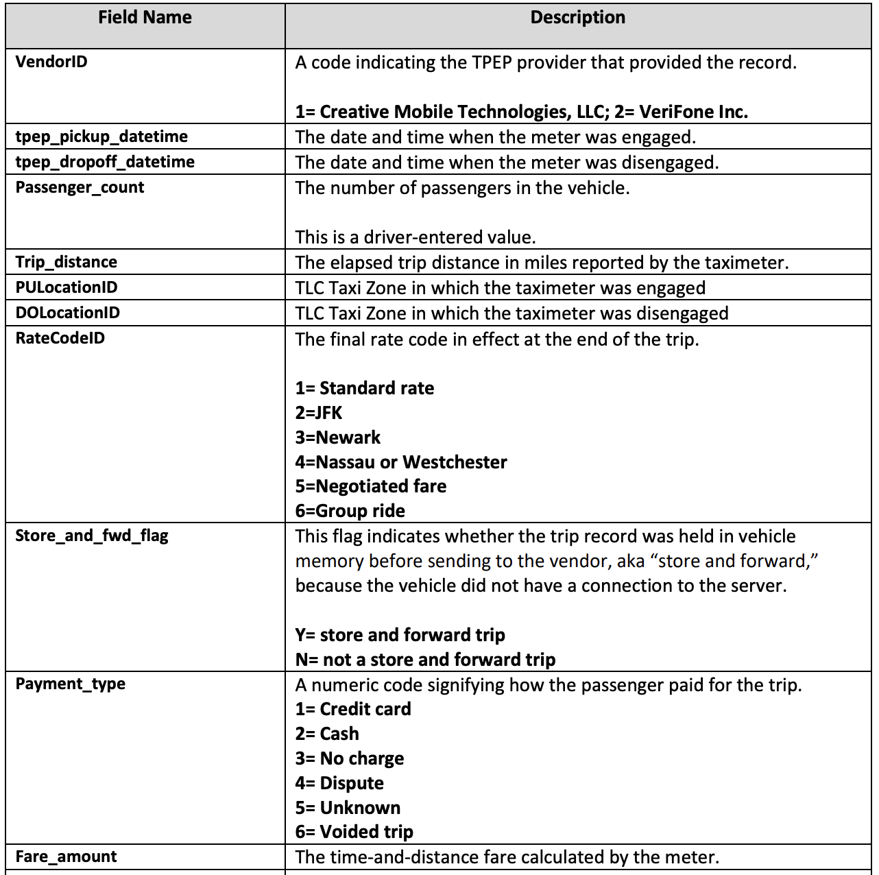
It is in fact in miles. The length of the United States is about 3000 miles, so this enterprising taxi travelled the entire US about 130 times.
The data dictionary tells us a lot of other useful things - for example, the Payment_type column should help us find disputed, voided, and other invalid charges.
Basic Cleaning
So what should we do? I'm thinking we look at more recent data, say anything 2020 and after. Let's get rid of anything with more than 3000 miles, and let's also get rid of rows with unreasonable negative numbers - eg. negative total amounts, tolls, etc. We can get rid of rows where the Payment_type is No Charge, Dispute, Voided, etc.
The trouble is if we just get rid of the negative amounts and disputes then we're leaving the corresponding equally invalid positive amount in the data - eg. if we drop the row that has the -\$1301.85 amount we'll still have the \$1301.85 row in our data.
We'll have to figure out how to drop both: for each of the negative numbers, we'll need to find the corresponding positive amount and get rid of those rows too.
Let's take a look at the outlier data and see if spot any clues for how to get rid of them.
(
    data
    .filter(
        (pl.col("total_amount") > 1300) |
        (pl.col("total_amount") < -1300)
    )
)
| VendorID | tpep_pickup_datetime | tpep_dropoff_datetime | passenger_count | trip_distance | RatecodeID | store_and_fwd_flag | PULocationID | DOLocationID | payment_type | fare_amount | extra | mta_tax | tip_amount | tolls_amount | improvement_surcharge | total_amount | congestion_surcharge | airport_fee |
|---|---|---|---|---|---|---|---|---|---|---|---|---|---|---|---|---|---|---|
| i64 | datetime[ns] | datetime[ns] | f64 | f64 | f64 | str | i64 | i64 | i64 | f64 | f64 | f64 | f64 | f64 | f64 | f64 | f64 | f64 |
| 2 | 2022-10-12 07:00:43 | 2022-10-12 12:31:57 | 4.0 | 259.33 | 4.0 | "N" | 39 | 265 | 2 | -1294.5 | 0.0 | -0.5 | 0.0 | -6.55 | -0.3 | -1301.85 | 0.0 | 0.0 |
| 2 | 2022-10-12 07:00:43 | 2022-10-12 12:31:57 | 4.0 | 259.33 | 4.0 | "N" | 39 | 265 | 2 | 1294.5 | 0.0 | 0.5 | 0.0 | 6.55 | 0.3 | 1301.85 | 0.0 | 0.0 |
The payment type is 2, which is cash. Somebody paid $1300 in cash, then got it handed back to him. I was hoping the payment type would be Voided or something reasonable.
Getting rid of these invalid pairs is going to be a bit painful - we'll have to find each invalid ride and also find its pair.
Before we do that, let's see if the problems still exists in data we care about, which is data from 2020 onwards.
data.filter( pl.col("tpep_pickup_datetime") > "2020" ).describe()
Warning: Comparing date/datetime/time column to string value, this will lead to string comparison and is unlikely what you want.
If this is intended, consider using an explicit cast to silence this warning.
| describe | VendorID | tpep_pickup_datetime | tpep_dropoff_datetime | passenger_count | trip_distance | RatecodeID | store_and_fwd_flag | PULocationID | DOLocationID | payment_type | fare_amount | extra | mta_tax | tip_amount | tolls_amount | improvement_surcharge | total_amount | congestion_surcharge | airport_fee |
|---|---|---|---|---|---|---|---|---|---|---|---|---|---|---|---|---|---|---|---|
| str | f64 | str | str | f64 | f64 | f64 | str | f64 | f64 | f64 | f64 | f64 | f64 | f64 | f64 | f64 | f64 | f64 | f64 |
| "count" | 3.675407e6 | "3675407" | "3675407" | 3.675407e6 | 3.675407e6 | 3.675407e6 | "3675407" | 3.675407e6 | 3.675407e6 | 3.675407e6 | 3.675407e6 | 3.675407e6 | 3.675407e6 | 3.675407e6 | 3.675407e6 | 3.675407e6 | 3.675407e6 | 3.675407e6 | 3.675407e6 |
| "null_count" | 0.0 | "0" | "0" | 133021.0 | 0.0 | 133021.0 | "133021" | 0.0 | 0.0 | 0.0 | 0.0 | 0.0 | 0.0 | 0.0 | 0.0 | 0.0 | 0.0 | 133021.0 | 133021.0 |
| "mean" | 1.720442 | null | null | 1.384694 | 6.206973 | 1.424337 | null | 165.498365 | 162.891771 | 1.188275 | 15.299922 | 0.987794 | 0.487229 | 2.859248 | 0.583304 | 0.295531 | 22.247504 | 2.280621 | 0.103127 |
| "std" | 0.480032 | null | null | 0.930231 | 640.824117 | 5.685594 | null | 65.213049 | 70.197445 | 0.540651 | 14.674414 | 1.242828 | 0.101155 | 3.374169 | 2.111966 | 0.051038 | 18.368208 | 0.757839 | 0.347973 |
| "min" | 1.0 | "2022-09-30 14:06:36.000000000" | "2022-09-30 14:23:04.000000000" | 0.0 | 0.0 | 1.0 | "N" | 1.0 | 1.0 | 0.0 | -1294.5 | -22.18 | -0.5 | -100.01 | -70.0 | -0.3 | -1301.85 | -2.5 | -1.25 |
| "max" | 6.0 | "2022-11-01 01:27:35.000000000" | "2022-11-03 17:26:46.000000000" | 9.0 | 389678.46 | 99.0 | "Y" | 265.0 | 265.0 | 4.0 | 1294.5 | 10.8 | 25.48 | 500.0 | 516.75 | 1.0 | 1301.85 | 2.5 | 1.25 |
| "median" | 2.0 | null | null | 1.0 | 1.9 | 1.0 | null | 162.0 | 162.0 | 1.0 | 10.5 | 0.5 | 0.5 | 2.22 | 0.0 | 0.3 | 16.55 | 2.5 | 0.0 |
That didn't work - our min tpep_pickup_datetime is 2022-09-30 (I was expecting 2020). I guess I can't filter a datetime column (tpep_pickup_datetime) using a string ("2020"). Makes sense, let's fix it.
from datetime import datetime
start_date = datetime(2020,1,1,0,0,0)
print(f"Filtering data to start at {start_date}")
data.filter( pl.col("tpep_pickup_datetime") > start_date ).describe()
Filtering data to start at 2020-01-01 00:00:00
| describe | VendorID | tpep_pickup_datetime | tpep_dropoff_datetime | passenger_count | trip_distance | RatecodeID | store_and_fwd_flag | PULocationID | DOLocationID | payment_type | fare_amount | extra | mta_tax | tip_amount | tolls_amount | improvement_surcharge | total_amount | congestion_surcharge | airport_fee |
|---|---|---|---|---|---|---|---|---|---|---|---|---|---|---|---|---|---|---|---|
| str | f64 | str | str | f64 | f64 | f64 | str | f64 | f64 | f64 | f64 | f64 | f64 | f64 | f64 | f64 | f64 | f64 | f64 |
| "count" | 3.675407e6 | "3675407" | "3675407" | 3.675407e6 | 3.675407e6 | 3.675407e6 | "3675407" | 3.675407e6 | 3.675407e6 | 3.675407e6 | 3.675407e6 | 3.675407e6 | 3.675407e6 | 3.675407e6 | 3.675407e6 | 3.675407e6 | 3.675407e6 | 3.675407e6 | 3.675407e6 |
| "null_count" | 0.0 | "0" | "0" | 133021.0 | 0.0 | 133021.0 | "133021" | 0.0 | 0.0 | 0.0 | 0.0 | 0.0 | 0.0 | 0.0 | 0.0 | 0.0 | 0.0 | 133021.0 | 133021.0 |
| "mean" | 1.720442 | null | null | 1.384694 | 6.206973 | 1.424337 | null | 165.498365 | 162.891771 | 1.188275 | 15.299922 | 0.987794 | 0.487229 | 2.859248 | 0.583304 | 0.295531 | 22.247504 | 2.280621 | 0.103127 |
| "std" | 0.480032 | null | null | 0.930231 | 640.824117 | 5.685594 | null | 65.213049 | 70.197445 | 0.540651 | 14.674414 | 1.242828 | 0.101155 | 3.374169 | 2.111966 | 0.051038 | 18.368208 | 0.757839 | 0.347973 |
| "min" | 1.0 | "2022-09-30 14:06:36.000000000" | "2022-09-30 14:23:04.000000000" | 0.0 | 0.0 | 1.0 | "N" | 1.0 | 1.0 | 0.0 | -1294.5 | -22.18 | -0.5 | -100.01 | -70.0 | -0.3 | -1301.85 | -2.5 | -1.25 |
| "max" | 6.0 | "2022-11-01 01:27:35.000000000" | "2022-11-03 17:26:46.000000000" | 9.0 | 389678.46 | 99.0 | "Y" | 265.0 | 265.0 | 4.0 | 1294.5 | 10.8 | 25.48 | 500.0 | 516.75 | 1.0 | 1301.85 | 2.5 | 1.25 |
| "median" | 2.0 | null | null | 1.0 | 1.9 | 1.0 | null | 162.0 | 162.0 | 1.0 | 10.5 | 0.5 | 0.5 | 2.22 | 0.0 | 0.3 | 16.55 | 2.5 | 0.0 |
My min tpep_pickup_datetime is still 2022-09-30 (I was expecting 2020). What's going on? Maybe our data is only for Octover 2022 after all, and the 2008 date I was seeing was spurious? Note that we had 3675411 data points before we filtered by date and now we have 3675407 data points (I'm getting this by looking at the count field for tpep_pickup_datetime). Our date filtering only got rid of 4 data points. So we're looking only at October 2022 data with a couple of spurious data points thrown in.
I'm curious what the data with bad dates look like.
(
    data
    .filter(
        (pl.col("tpep_pickup_datetime") < start_date)
    )
)
| VendorID | tpep_pickup_datetime | tpep_dropoff_datetime | passenger_count | trip_distance | RatecodeID | store_and_fwd_flag | PULocationID | DOLocationID | payment_type | fare_amount | extra | mta_tax | tip_amount | tolls_amount | improvement_surcharge | total_amount | congestion_surcharge | airport_fee |
|---|---|---|---|---|---|---|---|---|---|---|---|---|---|---|---|---|---|---|
| i64 | datetime[ns] | datetime[ns] | f64 | f64 | f64 | str | i64 | i64 | i64 | f64 | f64 | f64 | f64 | f64 | f64 | f64 | f64 | f64 |
| 2 | 2009-01-01 01:57:50 | 2009-01-01 02:20:59 | 1.0 | 7.84 | 1.0 | "N" | 161 | 264 | 2 | 22.0 | 0.5 | 0.5 | 0.0 | 0.0 | 0.3 | 23.3 | 0.0 | 0.0 |
| 2 | 2008-12-31 23:02:01 | 2009-01-01 19:08:45 | 1.0 | 22.93 | 1.0 | "N" | 132 | 25 | 1 | 63.0 | 0.0 | 0.5 | 13.01 | 0.0 | 0.3 | 78.06 | 0.0 | 1.25 |
| 2 | 2008-12-31 23:02:02 | 2009-01-01 20:14:39 | 1.0 | 0.0 | 2.0 | "N" | 231 | 231 | 1 | 52.0 | 0.0 | 0.5 | 10.0 | 0.0 | 0.3 | 66.55 | 2.5 | 1.25 |
| 2 | 2009-01-01 00:02:31 | 2009-01-01 17:02:49 | 1.0 | 8.11 | 1.0 | "N" | 138 | 186 | 1 | 35.5 | 1.0 | 0.5 | 9.52 | 6.55 | 0.3 | 57.12 | 2.5 | 1.25 |
Finding bad pairs
I don't see any obvious ways to correlate the bad pairs - the rows don't have IDs, there is no cab ID, and the payment method field doesn't give us much either. We'll have to data science.
Let's try this: - Find negative data points - For each negative data point, find a data point with the same amount but positive that also matches other parameters such as date and pick up / drop off location
(
    data
    .filter( pl.col("fare_amount") < 0)
)
| VendorID | tpep_pickup_datetime | tpep_dropoff_datetime | passenger_count | trip_distance | RatecodeID | store_and_fwd_flag | PULocationID | DOLocationID | payment_type | fare_amount | extra | mta_tax | tip_amount | tolls_amount | improvement_surcharge | total_amount | congestion_surcharge | airport_fee |
|---|---|---|---|---|---|---|---|---|---|---|---|---|---|---|---|---|---|---|
| i64 | datetime[ns] | datetime[ns] | f64 | f64 | f64 | str | i64 | i64 | i64 | f64 | f64 | f64 | f64 | f64 | f64 | f64 | f64 | f64 |
| 2 | 2022-10-01 00:52:07 | 2022-10-01 01:02:44 | 1.0 | 2.83 | 1.0 | "N" | 141 | 79 | 4 | -10.5 | -0.5 | -0.5 | 0.0 | 0.0 | -0.3 | -14.3 | -2.5 | 0.0 |
| 2 | 2022-10-01 00:29:57 | 2022-10-01 00:34:37 | 1.0 | 0.31 | 1.0 | "N" | 264 | 264 | 4 | -4.5 | -0.5 | -0.5 | 0.0 | 0.0 | -0.3 | -8.3 | -2.5 | 0.0 |
| 2 | 2022-10-01 00:31:37 | 2022-10-01 00:32:53 | 1.0 | 0.31 | 1.0 | "N" | 138 | 138 | 4 | -3.0 | -0.5 | -0.5 | 0.0 | 0.0 | -0.3 | -5.55 | 0.0 | -1.25 |
| 2 | 2022-10-01 00:46:38 | 2022-10-01 00:46:44 | 1.0 | 0.0 | 2.0 | "N" | 249 | 249 | 3 | -52.0 | 0.0 | -0.5 | 0.0 | 0.0 | -0.3 | -55.3 | -2.5 | 0.0 |
| 2 | 2022-10-01 00:06:08 | 2022-10-01 00:48:23 | 1.0 | 17.05 | 1.0 | "N" | 238 | 175 | 4 | -50.5 | -0.5 | -0.5 | 0.0 | -6.55 | -0.3 | -60.85 | -2.5 | 0.0 |
| 2 | 2022-10-01 00:40:58 | 2022-10-01 00:56:33 | 1.0 | 2.7 | 5.0 | "N" | 148 | 90 | 4 | -27.31 | 0.0 | -0.5 | 0.0 | 0.0 | -0.3 | -30.61 | -2.5 | 0.0 |
| 2 | 2022-10-01 00:43:19 | 2022-10-01 00:44:02 | 1.0 | 0.02 | 1.0 | "N" | 90 | 90 | 3 | -2.5 | -0.5 | -0.5 | 0.0 | 0.0 | -0.3 | -6.3 | -2.5 | 0.0 |
| 2 | 2022-10-01 00:12:32 | 2022-10-01 00:12:51 | 1.0 | 0.0 | 1.0 | "N" | 48 | 48 | 4 | -2.5 | -0.5 | -0.5 | 0.0 | 0.0 | -0.3 | -6.3 | -2.5 | 0.0 |
| 2 | 2022-10-01 00:12:24 | 2022-10-01 00:13:06 | 1.0 | 0.33 | 1.0 | "N" | 138 | 138 | 4 | -3.0 | -0.5 | -0.5 | 0.0 | 0.0 | -0.3 | -5.55 | 0.0 | -1.25 |
| 2 | 2022-10-01 00:39:21 | 2022-10-01 00:40:07 | 4.0 | 0.15 | 1.0 | "N" | 230 | 230 | 3 | -2.5 | -0.5 | -0.5 | 0.0 | 0.0 | -0.3 | -6.3 | -2.5 | 0.0 |
| 2 | 2022-10-01 00:08:25 | 2022-10-01 00:21:22 | 2.0 | 1.46 | 1.0 | "N" | 79 | 211 | 4 | -9.5 | -0.5 | -0.5 | 0.0 | 0.0 | -0.3 | -13.3 | -2.5 | 0.0 |
| 2 | 2022-10-01 00:45:01 | 2022-10-01 01:18:01 | 2.0 | 2.35 | 1.0 | "N" | 79 | 249 | 4 | -13.0 | -0.5 | -0.5 | 0.0 | 0.0 | -0.3 | -16.8 | -2.5 | 0.0 |
| ... | ... | ... | ... | ... | ... | ... | ... | ... | ... | ... | ... | ... | ... | ... | ... | ... | ... | ... |
| 2 | 2022-10-06 16:17:49 | 2022-10-06 16:20:42 | null | 0.28 | null | null | 79 | 107 | 0 | -95.68 | 0.0 | 0.5 | 15.22 | 0.0 | 0.3 | -77.16 | null | null |
| 2 | 2022-10-10 12:27:10 | 2022-10-10 12:56:00 | null | 60043.58 | null | null | 125 | 68 | 0 | -17.28 | 0.0 | -0.5 | -4.49 | 0.0 | 0.3 | -24.77 | null | null |
| 2 | 2022-10-13 21:55:30 | 2022-10-13 21:56:26 | null | 0.03 | null | null | 144 | 144 | 0 | -27.33 | 0.0 | 0.5 | 3.69 | 0.0 | 0.3 | -20.34 | null | null |
| 2 | 2022-10-13 22:44:00 | 2022-10-13 22:45:00 | null | 0.03 | null | null | 90 | 90 | 0 | -38.85 | 0.0 | 0.5 | 6.62 | 0.0 | 0.3 | -28.93 | null | null |
| 2 | 2022-10-14 03:26:00 | 2022-10-14 03:27:00 | null | 0.04 | null | null | 114 | 114 | 0 | -26.79 | 0.0 | 0.5 | 0.0 | 0.0 | 0.3 | -23.49 | null | null |
| 2 | 2022-10-16 04:52:00 | 2022-10-16 05:01:00 | null | 2.71 | null | null | 233 | 262 | 0 | -61.61 | 0.0 | 0.5 | 5.9 | 0.0 | 0.3 | -52.41 | null | null |
| 1 | 2022-10-18 13:06:39 | 2022-10-18 13:06:52 | null | 0.0 | null | null | 232 | 232 | 0 | -0.8 | 0.0 | 0.5 | 0.0 | 0.0 | 0.3 | 2.5 | null | null |
| 2 | 2022-10-19 01:55:00 | 2022-10-19 01:56:00 | null | 0.06 | null | null | 237 | 237 | 0 | -22.39 | 0.0 | 0.5 | 2.92 | 0.0 | 0.3 | -16.17 | null | null |
| 1 | 2022-10-22 19:35:59 | 2022-10-22 19:36:03 | null | 0.0 | null | null | 239 | 239 | 0 | -0.8 | 0.0 | 0.5 | 0.0 | 0.0 | 0.3 | 2.5 | null | null |
| 2 | 2022-10-25 07:40:00 | 2022-10-25 07:42:00 | null | 0.07 | null | null | 140 | 140 | 0 | -54.25 | 0.0 | 0.5 | 7.29 | 0.0 | 0.3 | -43.66 | null | null |
| 1 | 2022-10-28 09:13:07 | 2022-10-28 09:13:26 | null | 0.0 | null | null | 141 | 141 | 0 | -0.8 | 0.0 | 0.5 | 0.0 | 0.0 | 0.3 | 2.5 | null | null |
| 2 | 2022-10-29 07:33:24 | 2022-10-29 07:37:01 | null | 0.5 | null | null | 37 | 37 | 0 | -18.55 | 0.0 | 0.5 | 2.72 | 0.0 | 0.3 | -15.03 | null | null |
There's probably a clever way to do this, but my initial thought for getting rid of the corresponding positives is to create a new dataframe with the negative rows, then do an anti-join back to the original dataframe. An anti-join should find matching rows and remove them.
negative_data = (
    data
    .filter( pl.col("fare_amount") < 0)
).select(["tpep_pickup_datetime", "PULocationID", "fare_amount"])

negative_data
| tpep_pickup_datetime | PULocationID | fare_amount |
|---|---|---|
| datetime[ns] | i64 | f64 |
| 2022-10-01 00:52:07 | 141 | -10.5 |
| 2022-10-01 00:29:57 | 264 | -4.5 |
| 2022-10-01 00:31:37 | 138 | -3.0 |
| 2022-10-01 00:46:38 | 249 | -52.0 |
| 2022-10-01 00:06:08 | 238 | -50.5 |
| 2022-10-01 00:40:58 | 148 | -27.31 |
| 2022-10-01 00:43:19 | 90 | -2.5 |
| 2022-10-01 00:12:32 | 48 | -2.5 |
| 2022-10-01 00:12:24 | 138 | -3.0 |
| 2022-10-01 00:39:21 | 230 | -2.5 |
| 2022-10-01 00:08:25 | 79 | -9.5 |
| 2022-10-01 00:45:01 | 79 | -13.0 |
| ... | ... | ... |
| 2022-10-06 16:17:49 | 79 | -95.68 |
| 2022-10-10 12:27:10 | 125 | -17.28 |
| 2022-10-13 21:55:30 | 144 | -27.33 |
| 2022-10-13 22:44:00 | 90 | -38.85 |
| 2022-10-14 03:26:00 | 114 | -26.79 |
| 2022-10-16 04:52:00 | 233 | -61.61 |
| 2022-10-18 13:06:39 | 232 | -0.8 |
| 2022-10-19 01:55:00 | 237 | -22.39 |
| 2022-10-22 19:35:59 | 239 | -0.8 |
| 2022-10-25 07:40:00 | 140 | -54.25 |
| 2022-10-28 09:13:07 | 141 | -0.8 |
| 2022-10-29 07:33:24 | 37 | -18.55 |
I'm only grabbing a few columns for my negative_data dataframe, since all I'm going to use it for is to remove the corresponding positive rows from the original data. I'll try matching on the pick up date and pick up location.
Let's convert the negative amounts to positive so we can directly match them to their corresponding positive rows in the original data.
negative_data = negative_data.with_columns([
    (pl.col("fare_amount") * -1).alias("amount_positive")
])

negative_data
| tpep_pickup_datetime | PULocationID | fare_amount | amount_positive |
|---|---|---|---|
| datetime[ns] | i64 | f64 | f64 |
| 2022-10-01 00:52:07 | 141 | -10.5 | 10.5 |
| 2022-10-01 00:29:57 | 264 | -4.5 | 4.5 |
| 2022-10-01 00:31:37 | 138 | -3.0 | 3.0 |
| 2022-10-01 00:46:38 | 249 | -52.0 | 52.0 |
| 2022-10-01 00:06:08 | 238 | -50.5 | 50.5 |
| 2022-10-01 00:40:58 | 148 | -27.31 | 27.31 |
| 2022-10-01 00:43:19 | 90 | -2.5 | 2.5 |
| 2022-10-01 00:12:32 | 48 | -2.5 | 2.5 |
| 2022-10-01 00:12:24 | 138 | -3.0 | 3.0 |
| 2022-10-01 00:39:21 | 230 | -2.5 | 2.5 |
| 2022-10-01 00:08:25 | 79 | -9.5 | 9.5 |
| 2022-10-01 00:45:01 | 79 | -13.0 | 13.0 |
| ... | ... | ... | ... |
| 2022-10-06 16:17:49 | 79 | -95.68 | 95.68 |
| 2022-10-10 12:27:10 | 125 | -17.28 | 17.28 |
| 2022-10-13 21:55:30 | 144 | -27.33 | 27.33 |
| 2022-10-13 22:44:00 | 90 | -38.85 | 38.85 |
| 2022-10-14 03:26:00 | 114 | -26.79 | 26.79 |
| 2022-10-16 04:52:00 | 233 | -61.61 | 61.61 |
| 2022-10-18 13:06:39 | 232 | -0.8 | 0.8 |
| 2022-10-19 01:55:00 | 237 | -22.39 | 22.39 |
| 2022-10-22 19:35:59 | 239 | -0.8 | 0.8 |
| 2022-10-25 07:40:00 | 140 | -54.25 | 54.25 |
| 2022-10-28 09:13:07 | 141 | -0.8 | 0.8 |
| 2022-10-29 07:33:24 | 37 | -18.55 | 18.55 |
Now that we have a dataframe with the negative amounts converted to positive, we can join back to the original data, matching on the (now positive) fare amount and the pick up location. We'll do an anti-join, which gets rids of the rows that match. If Polars didn't have anti-join as an option we could have merged the new dataframe with the original data and dropped duplicate rows.
data.join(negative_data, on=("PULocationID", "fare_amount"), how="anti")
| VendorID | tpep_pickup_datetime | tpep_dropoff_datetime | passenger_count | trip_distance | RatecodeID | store_and_fwd_flag | PULocationID | DOLocationID | payment_type | fare_amount | extra | mta_tax | tip_amount | tolls_amount | improvement_surcharge | total_amount | congestion_surcharge | airport_fee |
|---|---|---|---|---|---|---|---|---|---|---|---|---|---|---|---|---|---|---|
| i64 | datetime[ns] | datetime[ns] | f64 | f64 | f64 | str | i64 | i64 | i64 | f64 | f64 | f64 | f64 | f64 | f64 | f64 | f64 | f64 |
| 1 | 2022-10-01 00:03:41 | 2022-10-01 00:18:39 | 1.0 | 1.7 | 1.0 | "N" | 249 | 107 | 1 | 9.5 | 3.0 | 0.5 | 2.65 | 0.0 | 0.3 | 15.95 | 2.5 | 0.0 |
| 2 | 2022-10-01 00:14:30 | 2022-10-01 00:19:48 | 2.0 | 0.72 | 1.0 | "N" | 151 | 238 | 2 | 5.5 | 0.5 | 0.5 | 0.0 | 0.0 | 0.3 | 9.3 | 2.5 | 0.0 |
| 2 | 2022-10-01 00:27:13 | 2022-10-01 00:37:41 | 1.0 | 1.74 | 1.0 | "N" | 238 | 166 | 1 | 9.0 | 0.5 | 0.5 | 2.06 | 0.0 | 0.3 | 12.36 | 0.0 | 0.0 |
| 1 | 2022-10-01 00:32:53 | 2022-10-01 00:38:55 | 0.0 | 1.3 | 1.0 | "N" | 142 | 239 | 1 | 6.5 | 3.0 | 0.5 | 2.05 | 0.0 | 0.3 | 12.35 | 2.5 | 0.0 |
| 1 | 2022-10-01 00:44:55 | 2022-10-01 00:50:21 | 0.0 | 1.0 | 1.0 | "N" | 238 | 166 | 1 | 6.0 | 0.5 | 0.5 | 1.8 | 0.0 | 0.3 | 9.1 | 0.0 | 0.0 |
| 1 | 2022-10-01 00:22:52 | 2022-10-01 00:52:14 | 1.0 | 6.8 | 1.0 | "Y" | 186 | 41 | 2 | 25.5 | 3.0 | 0.5 | 0.0 | 0.0 | 0.3 | 29.3 | 2.5 | 0.0 |
| 2 | 2022-10-01 00:33:19 | 2022-10-01 00:44:51 | 3.0 | 1.88 | 1.0 | "N" | 162 | 145 | 2 | 10.5 | 0.5 | 0.5 | 0.0 | 0.0 | 0.3 | 14.3 | 2.5 | 0.0 |
| 1 | 2022-10-01 00:02:42 | 2022-10-01 00:50:01 | 1.0 | 12.2 | 1.0 | "N" | 100 | 22 | 1 | 41.0 | 3.0 | 0.5 | 3.0 | 0.0 | 0.3 | 47.8 | 2.5 | 0.0 |
| 2 | 2022-10-01 00:06:35 | 2022-10-01 00:24:38 | 1.0 | 7.79 | 1.0 | "N" | 138 | 112 | 1 | 23.5 | 0.5 | 0.5 | 4.96 | 0.0 | 0.3 | 31.01 | 0.0 | 1.25 |
| 2 | 2022-10-01 00:29:25 | 2022-10-01 00:43:15 | 1.0 | 4.72 | 1.0 | "N" | 145 | 75 | 1 | 14.5 | 0.5 | 0.5 | 1.5 | 0.0 | 0.3 | 19.8 | 2.5 | 0.0 |
| 1 | 2022-10-01 00:01:55 | 2022-10-01 00:20:16 | 1.0 | 8.8 | 1.0 | "N" | 138 | 236 | 1 | 26.0 | 4.25 | 0.5 | 5.64 | 6.55 | 0.3 | 43.24 | 2.5 | 1.25 |
| 1 | 2022-10-01 00:27:48 | 2022-10-01 00:59:50 | 1.0 | 8.6 | 1.0 | "N" | 140 | 36 | 1 | 29.5 | 3.0 | 0.5 | 6.0 | 0.0 | 0.3 | 39.3 | 2.5 | 0.0 |
| ... | ... | ... | ... | ... | ... | ... | ... | ... | ... | ... | ... | ... | ... | ... | ... | ... | ... | ... |
| 2 | 2022-10-31 23:30:42 | 2022-10-31 23:40:16 | null | 1.7 | null | null | 158 | 90 | 0 | 9.95 | 0.0 | 0.5 | 2.93 | 0.0 | 0.3 | 16.18 | null | null |
| 1 | 2022-10-31 23:42:05 | 2022-11-01 00:13:58 | null | 17.5 | null | null | 132 | 68 | 0 | 52.0 | 1.25 | 0.5 | 9.46 | 6.55 | 0.3 | 72.56 | null | null |
| 2 | 2022-10-31 23:52:34 | 2022-11-01 00:23:32 | null | 12.6 | null | null | 116 | 37 | 0 | 40.67 | 0.0 | 0.5 | 5.26 | 6.55 | 0.3 | 53.28 | null | null |
| 2 | 2022-10-31 23:16:12 | 2022-10-31 23:32:36 | null | 6.23 | null | null | 158 | 166 | 0 | 22.5 | 0.0 | 0.5 | 5.67 | 0.0 | 0.3 | 31.47 | null | null |
| 2 | 2022-10-31 23:15:00 | 2022-10-31 23:20:00 | null | 0.72 | null | null | 142 | 142 | 0 | 9.95 | 0.0 | 0.5 | 2.92 | 0.0 | 0.3 | 16.17 | null | null |
| 1 | 2022-10-31 23:20:21 | 2022-10-31 23:34:15 | null | 2.7 | null | null | 163 | 68 | 0 | 12.0 | 0.5 | 0.5 | 3.95 | 0.0 | 0.3 | 19.75 | null | null |
| 2 | 2022-10-31 23:45:37 | 2022-11-01 00:00:39 | null | 2.45 | null | null | 249 | 162 | 0 | 11.97 | 0.0 | 0.5 | 3.39 | 0.0 | 0.3 | 18.66 | null | null |
| 2 | 2022-10-31 23:56:35 | 2022-11-01 00:10:11 | null | 2.25 | null | null | 137 | 50 | 0 | 12.68 | 0.0 | 0.5 | 3.16 | 0.0 | 0.3 | 19.14 | null | null |
| 2 | 2022-10-31 23:22:00 | 2022-10-31 23:28:00 | null | 1.22 | null | null | 142 | 161 | 0 | 10.0 | 0.0 | 0.5 | 1.0 | 0.0 | 0.3 | 14.3 | null | null |
| 2 | 2022-10-31 23:25:00 | 2022-10-31 23:48:00 | null | 4.7 | null | null | 186 | 45 | 0 | 19.07 | 0.0 | 0.5 | 4.97 | 0.0 | 0.3 | 27.34 | null | null |
| 2 | 2022-10-31 23:32:54 | 2022-10-31 23:33:02 | null | 0.0 | null | null | 264 | 263 | 0 | 16.82 | 0.0 | 0.5 | 4.58 | 0.0 | 0.3 | 22.2 | null | null |
| 1 | 2022-10-31 23:21:34 | 2022-10-31 23:32:42 | null | 0.0 | null | null | 166 | 116 | 0 | 8.93 | 0.0 | 0.5 | 0.0 | 0.0 | 0.3 | 9.73 | null | null |
Did that work? Let's see how many rows that got rid of. After the anti-join we end up with 3649512 rows. We had and 25899 rows with negative values.
n_rows_original = data.shape[0]
n_rows_negative = negative_data.shape[0]
print(f"We are expecting {n_rows_original - n_rows_negative} rows if our removal worked perfectly")
We are expecting 3649512 rows if our removal worked perfectly
Sure enough the result of the anti-join has 3649512 rows (you can see that from the shape output a few cells above), so our method is working well. We should sanity check to make sure it's working as expected, but for now let's assume all is well.
We can now do our final cleaning: we'll get rid of the negative and corresponding positive rows, get rid of anything where the mileage is over 3000 miles, remove dates that are out of range, and get rid of rows with unknown pick up and drop off locations:
clean_data = (
    data
    .join(negative_data, on=("PULocationID", "fare_amount"), how="anti")
    .filter( pl.col("fare_amount") >= 0)
    .filter( pl.col("trip_distance") <= 3000 )
    .filter( pl.col("tpep_pickup_datetime") >= start_date )
    .filter(
        (pl.col("PULocationID") != 265) &
        (pl.col("DOLocationID") != 265)
    )
)

clean_data
| VendorID | tpep_pickup_datetime | tpep_dropoff_datetime | passenger_count | trip_distance | RatecodeID | store_and_fwd_flag | PULocationID | DOLocationID | payment_type | fare_amount | extra | mta_tax | tip_amount | tolls_amount | improvement_surcharge | total_amount | congestion_surcharge | airport_fee |
|---|---|---|---|---|---|---|---|---|---|---|---|---|---|---|---|---|---|---|
| i64 | datetime[ns] | datetime[ns] | f64 | f64 | f64 | str | i64 | i64 | i64 | f64 | f64 | f64 | f64 | f64 | f64 | f64 | f64 | f64 |
| 1 | 2022-10-01 00:03:41 | 2022-10-01 00:18:39 | 1.0 | 1.7 | 1.0 | "N" | 249 | 107 | 1 | 9.5 | 3.0 | 0.5 | 2.65 | 0.0 | 0.3 | 15.95 | 2.5 | 0.0 |
| 2 | 2022-10-01 00:14:30 | 2022-10-01 00:19:48 | 2.0 | 0.72 | 1.0 | "N" | 151 | 238 | 2 | 5.5 | 0.5 | 0.5 | 0.0 | 0.0 | 0.3 | 9.3 | 2.5 | 0.0 |
| 2 | 2022-10-01 00:27:13 | 2022-10-01 00:37:41 | 1.0 | 1.74 | 1.0 | "N" | 238 | 166 | 1 | 9.0 | 0.5 | 0.5 | 2.06 | 0.0 | 0.3 | 12.36 | 0.0 | 0.0 |
| 1 | 2022-10-01 00:32:53 | 2022-10-01 00:38:55 | 0.0 | 1.3 | 1.0 | "N" | 142 | 239 | 1 | 6.5 | 3.0 | 0.5 | 2.05 | 0.0 | 0.3 | 12.35 | 2.5 | 0.0 |
| 1 | 2022-10-01 00:44:55 | 2022-10-01 00:50:21 | 0.0 | 1.0 | 1.0 | "N" | 238 | 166 | 1 | 6.0 | 0.5 | 0.5 | 1.8 | 0.0 | 0.3 | 9.1 | 0.0 | 0.0 |
| 1 | 2022-10-01 00:22:52 | 2022-10-01 00:52:14 | 1.0 | 6.8 | 1.0 | "Y" | 186 | 41 | 2 | 25.5 | 3.0 | 0.5 | 0.0 | 0.0 | 0.3 | 29.3 | 2.5 | 0.0 |
| 2 | 2022-10-01 00:33:19 | 2022-10-01 00:44:51 | 3.0 | 1.88 | 1.0 | "N" | 162 | 145 | 2 | 10.5 | 0.5 | 0.5 | 0.0 | 0.0 | 0.3 | 14.3 | 2.5 | 0.0 |
| 1 | 2022-10-01 00:02:42 | 2022-10-01 00:50:01 | 1.0 | 12.2 | 1.0 | "N" | 100 | 22 | 1 | 41.0 | 3.0 | 0.5 | 3.0 | 0.0 | 0.3 | 47.8 | 2.5 | 0.0 |
| 2 | 2022-10-01 00:06:35 | 2022-10-01 00:24:38 | 1.0 | 7.79 | 1.0 | "N" | 138 | 112 | 1 | 23.5 | 0.5 | 0.5 | 4.96 | 0.0 | 0.3 | 31.01 | 0.0 | 1.25 |
| 2 | 2022-10-01 00:29:25 | 2022-10-01 00:43:15 | 1.0 | 4.72 | 1.0 | "N" | 145 | 75 | 1 | 14.5 | 0.5 | 0.5 | 1.5 | 0.0 | 0.3 | 19.8 | 2.5 | 0.0 |
| 1 | 2022-10-01 00:01:55 | 2022-10-01 00:20:16 | 1.0 | 8.8 | 1.0 | "N" | 138 | 236 | 1 | 26.0 | 4.25 | 0.5 | 5.64 | 6.55 | 0.3 | 43.24 | 2.5 | 1.25 |
| 1 | 2022-10-01 00:27:48 | 2022-10-01 00:59:50 | 1.0 | 8.6 | 1.0 | "N" | 140 | 36 | 1 | 29.5 | 3.0 | 0.5 | 6.0 | 0.0 | 0.3 | 39.3 | 2.5 | 0.0 |
| ... | ... | ... | ... | ... | ... | ... | ... | ... | ... | ... | ... | ... | ... | ... | ... | ... | ... | ... |
| 2 | 2022-10-31 23:30:42 | 2022-10-31 23:40:16 | null | 1.7 | null | null | 158 | 90 | 0 | 9.95 | 0.0 | 0.5 | 2.93 | 0.0 | 0.3 | 16.18 | null | null |
| 1 | 2022-10-31 23:42:05 | 2022-11-01 00:13:58 | null | 17.5 | null | null | 132 | 68 | 0 | 52.0 | 1.25 | 0.5 | 9.46 | 6.55 | 0.3 | 72.56 | null | null |
| 2 | 2022-10-31 23:52:34 | 2022-11-01 00:23:32 | null | 12.6 | null | null | 116 | 37 | 0 | 40.67 | 0.0 | 0.5 | 5.26 | 6.55 | 0.3 | 53.28 | null | null |
| 2 | 2022-10-31 23:16:12 | 2022-10-31 23:32:36 | null | 6.23 | null | null | 158 | 166 | 0 | 22.5 | 0.0 | 0.5 | 5.67 | 0.0 | 0.3 | 31.47 | null | null |
| 2 | 2022-10-31 23:15:00 | 2022-10-31 23:20:00 | null | 0.72 | null | null | 142 | 142 | 0 | 9.95 | 0.0 | 0.5 | 2.92 | 0.0 | 0.3 | 16.17 | null | null |
| 1 | 2022-10-31 23:20:21 | 2022-10-31 23:34:15 | null | 2.7 | null | null | 163 | 68 | 0 | 12.0 | 0.5 | 0.5 | 3.95 | 0.0 | 0.3 | 19.75 | null | null |
| 2 | 2022-10-31 23:45:37 | 2022-11-01 00:00:39 | null | 2.45 | null | null | 249 | 162 | 0 | 11.97 | 0.0 | 0.5 | 3.39 | 0.0 | 0.3 | 18.66 | null | null |
| 2 | 2022-10-31 23:56:35 | 2022-11-01 00:10:11 | null | 2.25 | null | null | 137 | 50 | 0 | 12.68 | 0.0 | 0.5 | 3.16 | 0.0 | 0.3 | 19.14 | null | null |
| 2 | 2022-10-31 23:22:00 | 2022-10-31 23:28:00 | null | 1.22 | null | null | 142 | 161 | 0 | 10.0 | 0.0 | 0.5 | 1.0 | 0.0 | 0.3 | 14.3 | null | null |
| 2 | 2022-10-31 23:25:00 | 2022-10-31 23:48:00 | null | 4.7 | null | null | 186 | 45 | 0 | 19.07 | 0.0 | 0.5 | 4.97 | 0.0 | 0.3 | 27.34 | null | null |
| 2 | 2022-10-31 23:32:54 | 2022-10-31 23:33:02 | null | 0.0 | null | null | 264 | 263 | 0 | 16.82 | 0.0 | 0.5 | 4.58 | 0.0 | 0.3 | 22.2 | null | null |
| 1 | 2022-10-31 23:21:34 | 2022-10-31 23:32:42 | null | 0.0 | null | null | 166 | 116 | 0 | 8.93 | 0.0 | 0.5 | 0.0 | 0.0 | 0.3 | 9.73 | null | null |
How many rows of data did we get rid of?
data.shape[0] - clean_data.shape[0]
45288
clean_data.describe()
| describe | VendorID | tpep_pickup_datetime | tpep_dropoff_datetime | passenger_count | trip_distance | RatecodeID | store_and_fwd_flag | PULocationID | DOLocationID | payment_type | fare_amount | extra | mta_tax | tip_amount | tolls_amount | improvement_surcharge | total_amount | congestion_surcharge | airport_fee |
|---|---|---|---|---|---|---|---|---|---|---|---|---|---|---|---|---|---|---|---|
| str | f64 | str | str | f64 | f64 | f64 | str | f64 | f64 | f64 | f64 | f64 | f64 | f64 | f64 | f64 | f64 | f64 | f64 |
| "count" | 3.630123e6 | "3630123" | "3630123" | 3.630123e6 | 3.630123e6 | 3.630123e6 | "3630123" | 3.630123e6 | 3.630123e6 | 3.630123e6 | 3.630123e6 | 3.630123e6 | 3.630123e6 | 3.630123e6 | 3.630123e6 | 3.630123e6 | 3.630123e6 | 3.630123e6 | 3.630123e6 |
| "null_count" | 0.0 | "0" | "0" | 126893.0 | 0.0 | 126893.0 | "126893" | 0.0 | 0.0 | 0.0 | 0.0 | 0.0 | 0.0 | 0.0 | 0.0 | 0.0 | 0.0 | 126893.0 | 126893.0 |
| "mean" | 1.712003 | null | null | 1.384814 | 3.554337 | 1.413354 | null | 165.373444 | 162.575655 | 1.174523 | 15.200393 | 1.001434 | 0.494995 | 2.854254 | 0.571016 | 0.299767 | 22.190213 | 2.319343 | 0.103112 |
| "std" | 0.45283 | null | null | 0.931426 | 4.456602 | 5.684473 | null | 65.14861 | 70.034565 | 0.504213 | 13.14293 | 1.242161 | 0.0556 | 3.227445 | 2.036301 | 0.009334 | 16.768073 | 0.648033 | 0.343979 |
| "min" | 1.0 | "2022-09-30 14:06:36.000000000" | "2022-09-30 14:23:04.000000000" | 0.0 | 0.0 | 1.0 | "N" | 1.0 | 1.0 | 0.0 | 0.0 | -22.18 | -0.5 | 0.0 | 0.0 | -0.3 | -4.55 | -2.5 | -1.25 |
| "max" | 2.0 | "2022-11-01 01:27:35.000000000" | "2022-11-03 17:26:46.000000000" | 9.0 | 462.86 | 99.0 | "Y" | 264.0 | 264.0 | 4.0 | 950.0 | 10.8 | 25.48 | 500.0 | 516.75 | 0.3 | 950.3 | 2.5 | 1.25 |
| "median" | 2.0 | null | null | 1.0 | 1.9 | 1.0 | null | 162.0 | 162.0 | 1.0 | 10.5 | 0.5 | 0.5 | 2.25 | 0.0 | 0.3 | 16.55 | 2.5 | 0.0 |
That's looking better - we still have some negatives and other strange looking things, but you get a sense of how we'd approach getting rid of those. For next steps I'd probably filter more things that look incorrect, then I'd plot the data as a histogram and eyeball it to see if there's anything strange in there.
Let's stop there.
This was my first foray into Polars, so it's likely there are more polarsy ways of doing things - if you know of improvements please let me know.
Overall I really like Polars. It's fast and clean and the resulting code is easy on the eyes. I'm likely to use it in place of Pandas going forward.
Links
Modern Polars is quite nice with many examples.
Towards Data Science has a good article called Polars: Pandas DataFrame but Much Faster.
This article from Code Magazine has a lot of good Polars examples.
The Polars documentation page on Coming from Pandas is very useful if you have Pandas experience.
While we're at it, read this piece from a former cab driver on the ride he'll never forget.